4.4. Dual-axis Combo Chart in Python

This is a Notebook for the medium article Creating a dual-axis Combo Chart in Python

Please check out article for instructions

License: BSD 2-Clause

4.4.1. Version of packages used in this Notebook

%%capture
!pip install seaborn

import matplotlib as m
import numpy as np
import pandas as pd

# Make sure your package version >= them
print('matplotlib: ', m.__version__)
print('numpy: ', np.__version__)
print('pandas: ', pd.__version__)

matplotlib:  3.6.0
numpy:  1.23.2
pandas:  1.5.0

4.5. Tutorial

import matplotlib.pyplot as plt
import numpy as np
import pandas as pd

plt.style.use('seaborn')
# Needed for jupyter notebooks
%matplotlib inline
%config InlineBackend.figure_format = 'retina'
# Default figure size: 8 by 5
plt.rcParams['figure.figsize'] = (8, 5)

/var/folders/rp/c0_pxspj11g3dzxkc_qfxvdr0000gn/T/ipykernel_90922/2310884817.py:1: MatplotlibDeprecationWarning: The seaborn styles shipped by Matplotlib are deprecated since 3.6, as they no longer correspond to the styles shipped by seaborn. However, they will remain available as 'seaborn-v0_8-<style>'. Alternatively, directly use the seaborn API instead.
  plt.style.use('seaborn')

x = ['Jan', 'Feb', 'Mar', 'Apr', 'May', 'Jun', 'Jul', 'Aug', 'Sep', 'Oct', 'Nov', 'Dec']
#https://en.climate-data.org/europe/germany/bremen/bremen-82/
#1991-2021
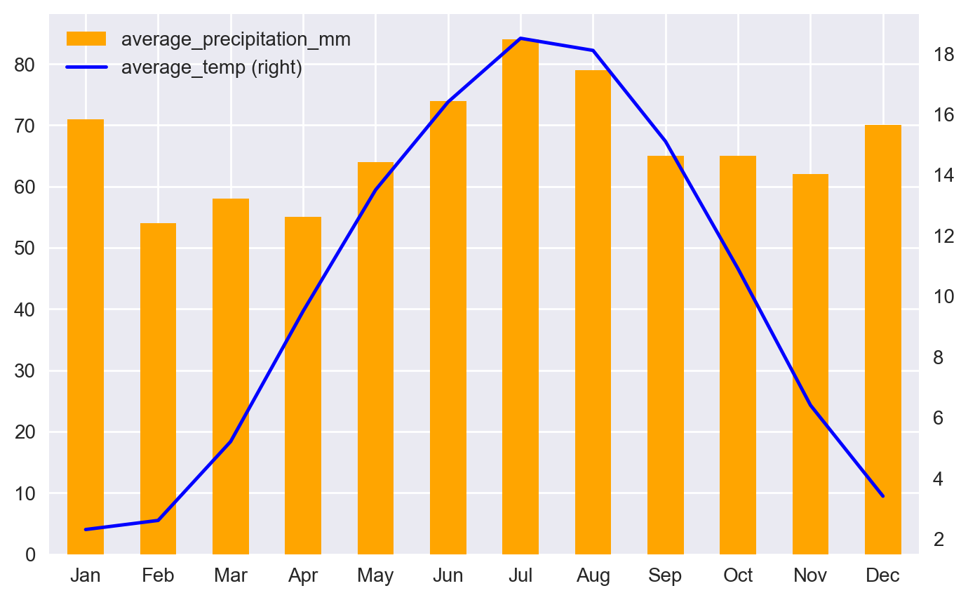
average_temp = [2.3, 2.6, 5.2, 9.5, 13.5, 16.4, 18.5, 18.1, 15.1, 10.9, 6.4, 3.4]
average_precipitation_mm = [71, 54, 58, 55, 64, 74, 84, 79, 65, 65, 62, 70]

bremen_climate = pd.DataFrame(
  {
    'average_temp': average_temp,
    'average_precipitation_mm': average_precipitation_mm
  }, 
  index=x
)

bremen_climate

	average_temp	average_precipitation_mm
Jan	2.3	71
Feb	2.6	54
Mar	5.2	58
Apr	9.5	55
May	13.5	64
Jun	16.4	74
Jul	18.5	84
Aug	18.1	79
Sep	15.1	65
Oct	10.9	65
Nov	6.4	62
Dec	3.4	70

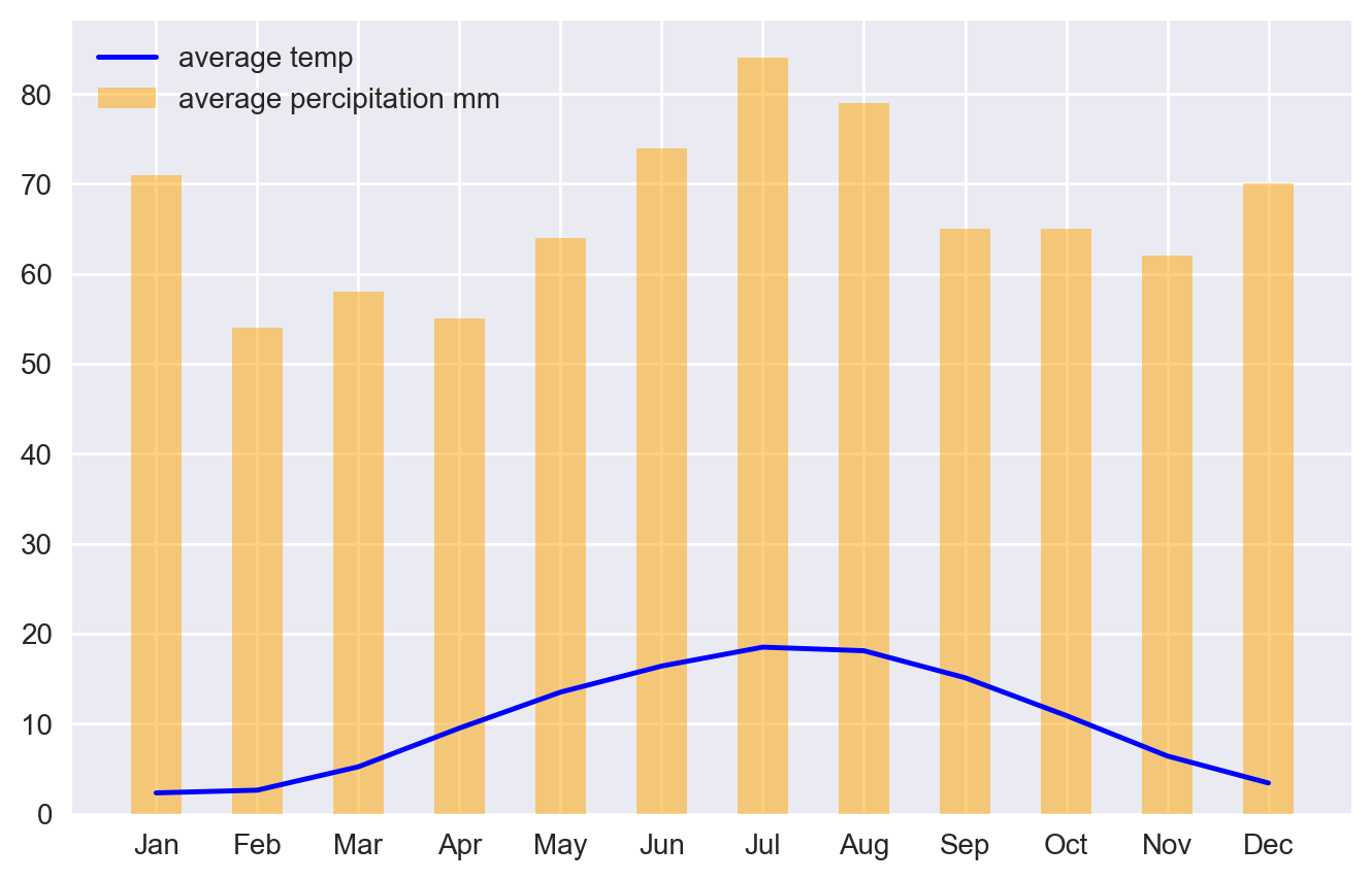
4.5.1. 1. Problem using the same axis

plt.plot(x, average_temp, "-b", label="average temp")
plt.bar(x, average_precipitation_mm, width=0.5, alpha=0.5, color='orange', label="average percipitation mm", )
plt.legend(loc="upper left")
plt.show()

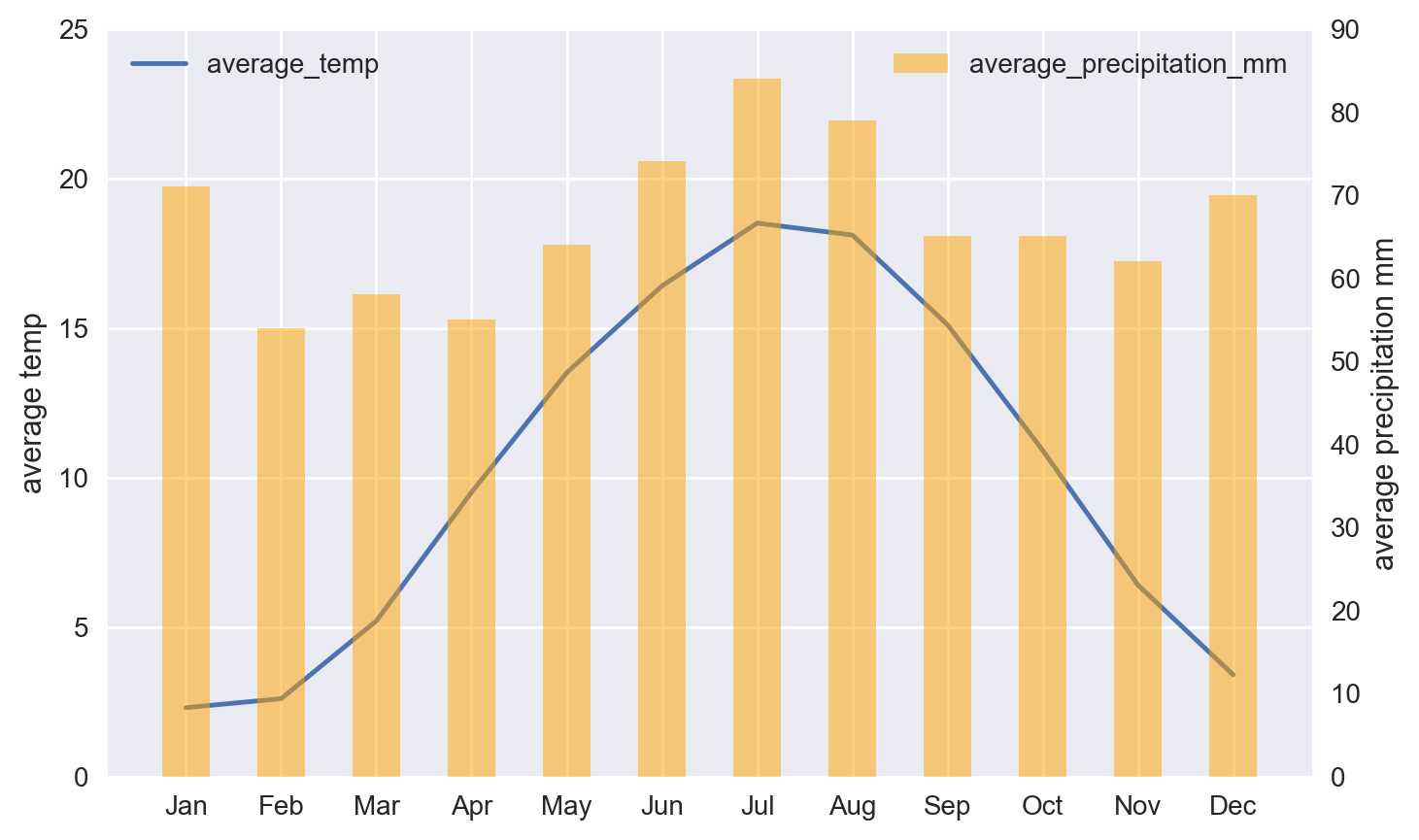
4.5.2. 2. Matplotlib - dual-axis combo chart

import matplotlib.pyplot as plt
import numpy as np
import pandas as pd

# Create figure and axis #1
fig, ax1 = plt.subplots()

# plot line chart on axis #1
ax1.plot(x, average_temp) 
ax1.set_ylabel('average temp')
ax1.set_ylim(0, 25)
ax1.legend(['average_temp'], loc="upper left")

# set up the 2nd axis
ax2 = ax1.twinx() 

# plot bar chart on axis #2
ax2.bar(x, average_precipitation_mm, width=0.5, alpha=0.5, color='orange')
ax2.grid(False) # turn off grid #2
ax2.set_ylabel('average precipitation mm')
ax2.set_ylim(0, 90)
ax2.legend(['average_precipitation_mm'], loc="upper right")

plt.show()

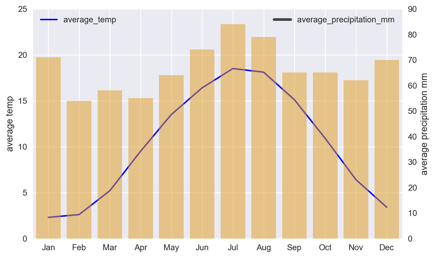
4.5.3. 2. Seaborn - dual-axis combo chart

bremen_climate_df = bremen_climate.reset_index()

import pandas as pd
import matplotlib
import matplotlib.pyplot as plt
import seaborn as sns

# plot line chart on axis #1
ax1 = sns.lineplot(
    x=bremen_climate.index, 
    y='average_temp', 
    data=bremen_climate, 
    sort=False, 
    color='blue'
)
ax1.set_ylabel('average temp')
ax1.set_ylim(0, 25)
ax1.legend(['average_temp'], loc="upper left")

# set up the 2nd axis
ax2 = ax1.twinx() 

# plot bar chart on axis #2
sns.barplot(
    x=bremen_climate.index, 
    y='average_precipitation_mm', 
    data=bremen_climate, 
    color='orange', 
    alpha=0.5, 
    ax = ax2       # Pre-existing axes for the plot
)
ax2.grid(False) # turn off grid #2
ax2.set_ylabel('average precipitation mm')
ax2.set_ylim(0, 90)
ax2.legend(['average_precipitation_mm'], loc="upper right")

plt.show()

bremen_climate

	average_temp	average_precipitation_mm
Jan	2.3	71
Feb	2.6	54
Mar	5.2	58
Apr	9.5	55
May	13.5	64
Jun	16.4	74
Jul	18.5	84
Aug	18.1	79
Sep	15.1	65
Oct	10.9	65
Nov	6.4	62
Dec	3.4	70

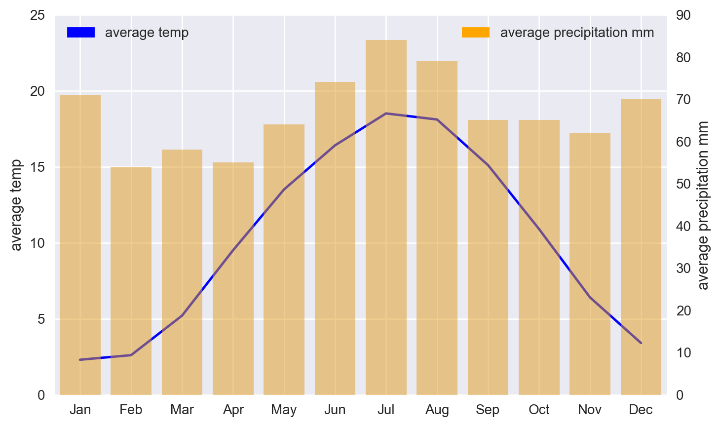
4.5.3.1. Fix legend color issue

import matplotlib.patches as mpatches

# plot line chart on axis #1
ax1 = sns.lineplot(
    x=bremen_climate.index,
    y='average_temp', 
    data=bremen_climate, 
    sort=False, 
    color='blue'
)
ax1.set_ylabel('average temp')
ax1.set_ylim(0, 25)
ax1_patch = mpatches.Patch(color='blue', label='average temp')
ax1.legend(handles=[ax1_patch], loc="upper left")

# set up the 2nd axis
ax2 = ax1.twinx() 

# plot bar chart on axis #2
sns.barplot(
    x=bremen_climate.index, 
    y='average_precipitation_mm', 
    data=bremen_climate, 
    color='orange', 
    alpha=0.5, 
    ax = ax2       # Pre-existing axes for the plot
)
ax2.grid(False) # turn off grid #2
ax2.set_ylabel('average precipitation mm')
ax2.set_ylim(0, 90)
ax2_patch = mpatches.Patch(color='orange', label='average precipitation mm')
ax2.legend(handles=[ax2_patch], loc="upper right")

plt.show()

4.5.4. 3. DataFrame plot

# Create the figure and axes object
fig, ax = plt.subplots()

# Plot the first x and y axes:
bremen_climate.plot(
    use_index=True, 
    kind='bar',
    y='average_precipitation_mm', 
    ax=ax, 
    color='orange'
) 

# Plot the second x and y axes. 
# By secondary_y = True a second y-axis is requested
bremen_climate.plot(
    use_index=True, 
    y='average_temp', 
    ax=ax, 
    secondary_y=True, 
    color='blue'
) 

plt.show()

4.5.5. Thanks for reading

This is a Notebook for the medium article Creating a dual-axis Combo Chart in Python

Please check out article for instructions

License: BSD 2-Clause